1.1 Change in Tandem

1.1.A

Function: a mathematical relation that maps a set of input values to a set of output values such that each input value is mapped to exactly one output value. The set of input values is called the domain of the function, and the set of output values is called the range of the function. The variable representing input values is called the independent variable, and the variable representing output values is called the dependent variable.

Function Rule: input and output values can be expressed graphically, numerically, analytically, or verbally.

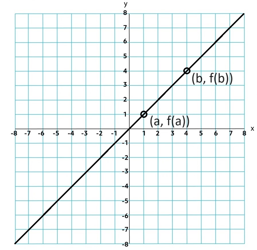
If a function is Increasing and variable a < b. then f(a) < f(b).

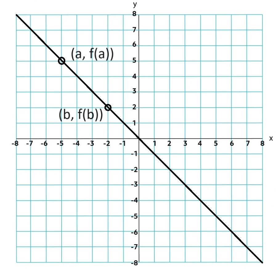
If a function is Decreasing and variable a < b. then f(a) > f(b).

1.1.B

Construct a graph representing two quantities that vary with respect to each other in a contextual scenario.

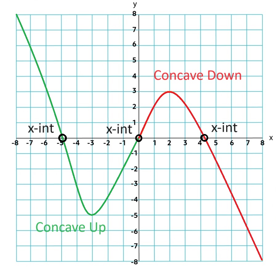
Concave Up: over an interval the rate of change is increasing

Concave Down: over an interval the rate of change is decreasing

Zeros: the input value when the output value is 0, aka x-intercept

1.2 Rates of Change

1.2.A

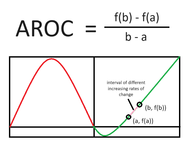
Average Rate of Change(AROC): ratio of the change in the output values to the change in input values over an interval. This rate of change in constant. The rate of change at a point can be approximated by AROC's of the function over small intervals.

1.2.B

Rates of Change: how two quantities vary together.

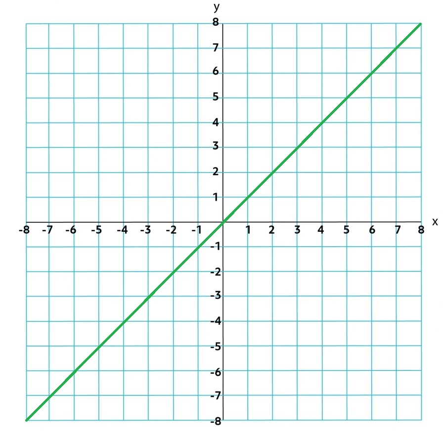
Positive rate of change: as a quantity increases or decreases, the other does the same

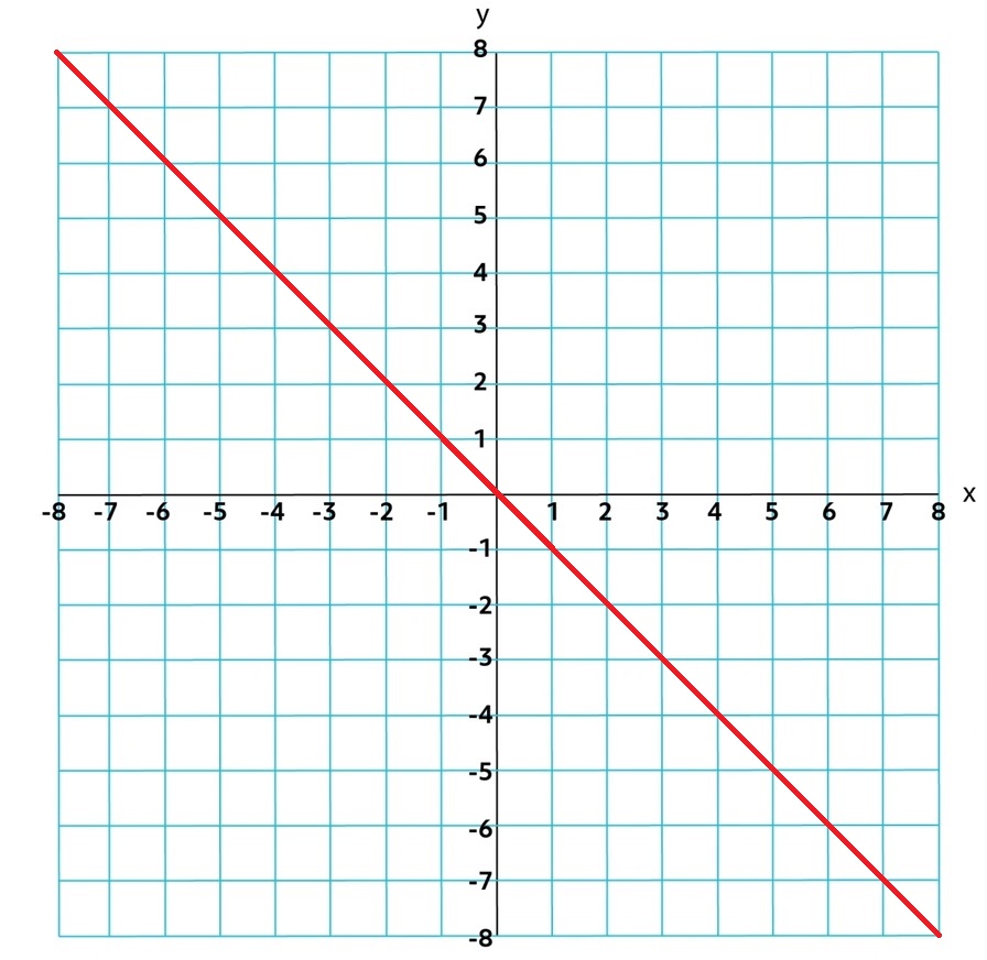
Negative rate of change: as a quantity increases, the other does decreases

1.3 Rates of Change in Linear and Quadratic Functions

1.3.A

Linear Function: the AROC over any length of input-value is constant

Quadratic Function: the AROC over consecutive equal-length input-value intervals can be given by a linear function.

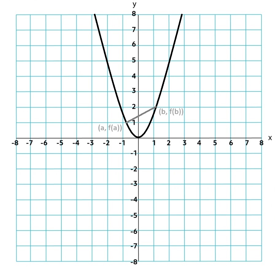
AROC over a closed interval [a, b] is the slope of the secant line from point (a, f(a)) to (b, f(b)).

1.3.B

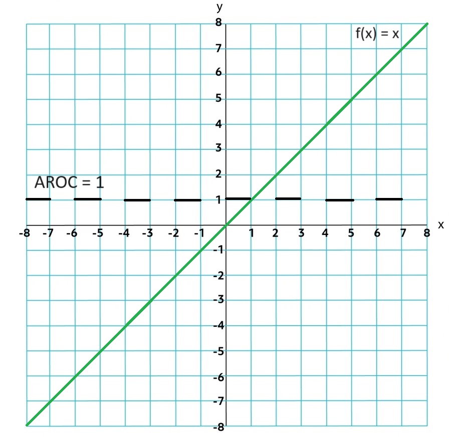
Linear Function: AROC over consecutive equal-length input-value intervals can be given by a constant function. They are changing at a rate of zero.

Quadratic Function: AROC over consecutive equal-length input-value intervals can be given by a linear function. They are changing at a constant rate.

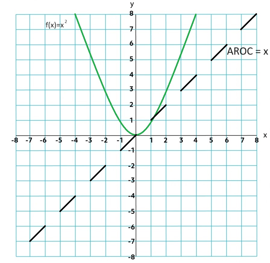
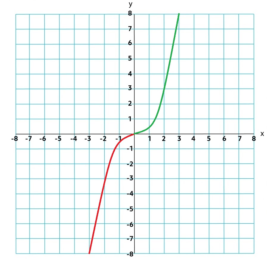
When the average rate of change over equal length input-value intervals is increasing for all small-length intervals, the graph of the function is concave up. When the average rate of change over equal-length input-value intervals is decreasing for all small-length intervals, the graph of the function is concave down.

1.4 Polynomial Functions and Rates of Change

1.4.A

Polynomial (analytical form): p(x) = a_nxⁿ + a_n−1xⁿ⁻¹ + a_n−2xⁿ⁻² +… + a₂x² + a₁x + a₀, where n is a positive integer, a_i is a real number for each i from 1 to n, and a_n is nonzero. Leading Term a_nxⁿ and Leading Coefficient a_n.

Ex. x³ + 3x² - 4x - 12 = 0

Where a polynomial function switches between increasing and decreasing, or at the included endpoint of a polynomial with a restricted domain, the polynomial function will have a local, or relative, maximum or minimum output value. Of all local maxima, the greatest is called the global, or absolute, maximum. Likewise, the least of all local minima is called the global, or absolute, minimum.

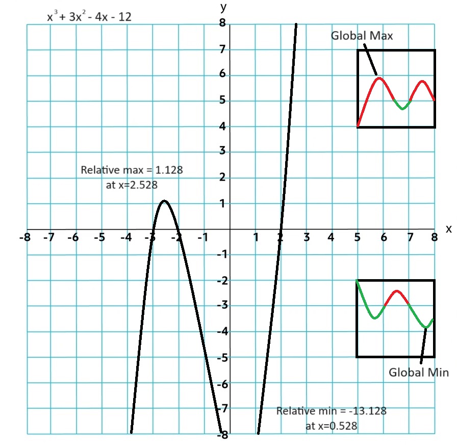
Even Function: always has an absolute min or max.

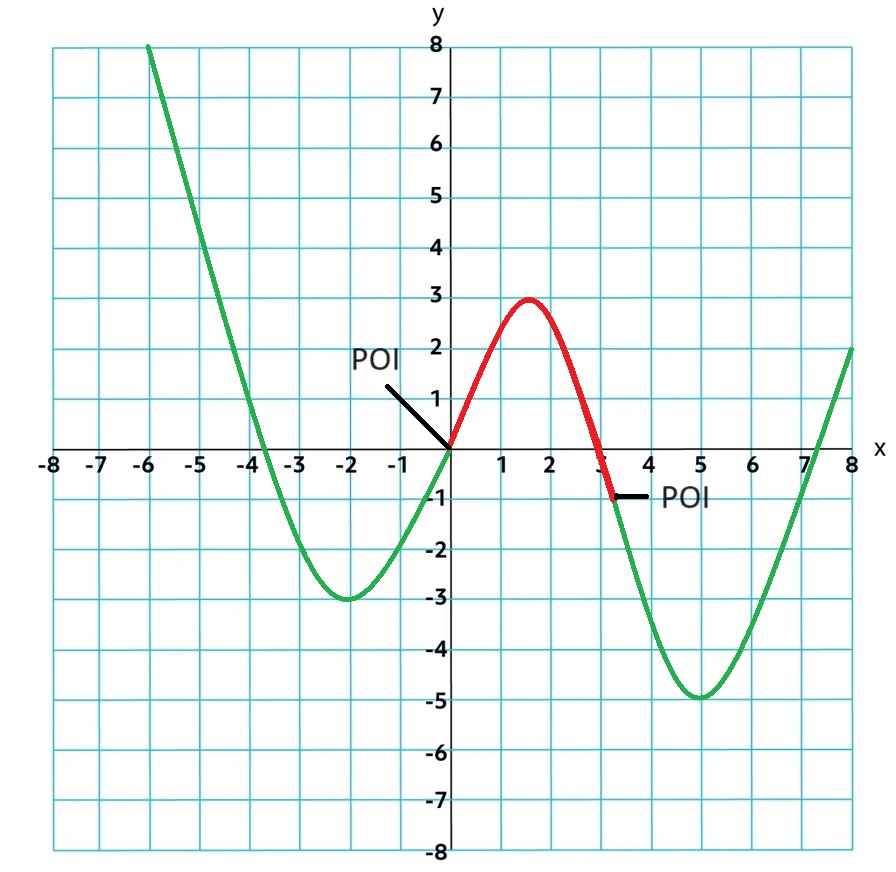
Points of Inflection: when the function goes from concave up to concave down

1.5 Polynomial Functions and Complex Zeros

1.5.A

Complex Zeros: refers to both the real and non-real numbers.

If p(a) = 0 then a is a zero of p. It is also an x-intercept at point (a, 0). If a is a real real number, then (x - a) is a linear factor.

Non-real zeros - in the form a+bi or its conjugate a-bi is a zero of p. These are not shown on the graph!!

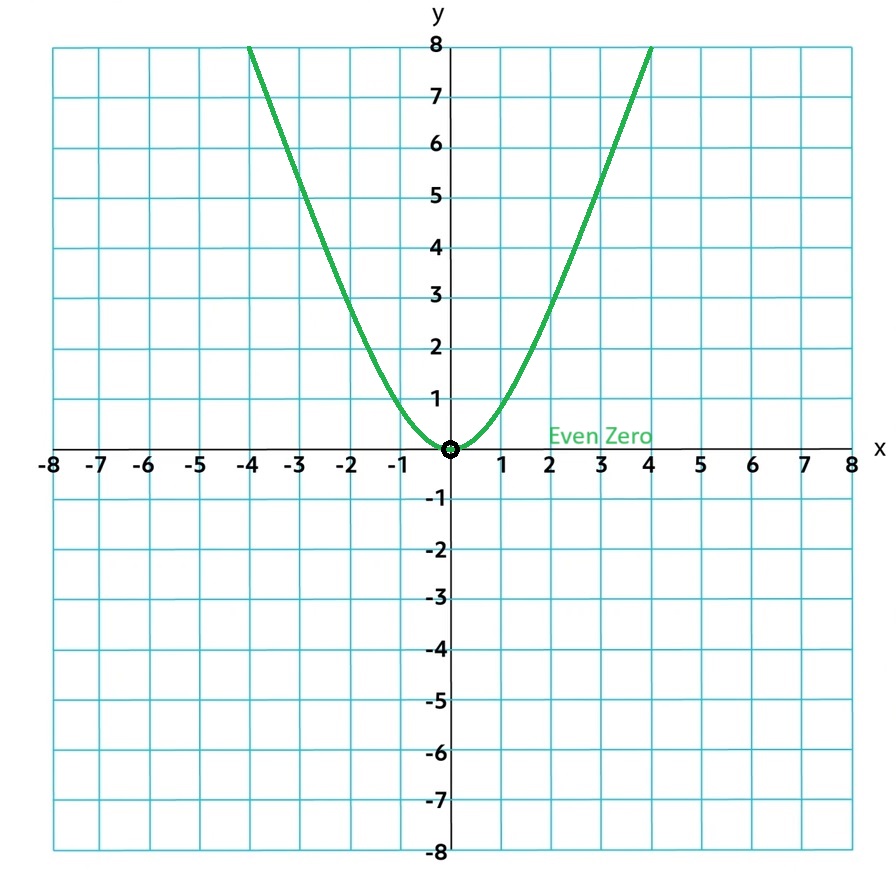
If the zero is even it will touch the x-axis

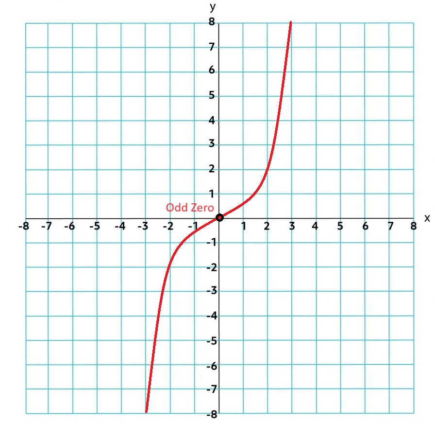
If the zero is odd it will go through the x-axis

Degree is always equal to the number of zeros!

1.5.B

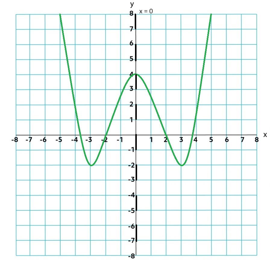
If the function is even it have symmetry across the y-axis. f(-x) = f(x)

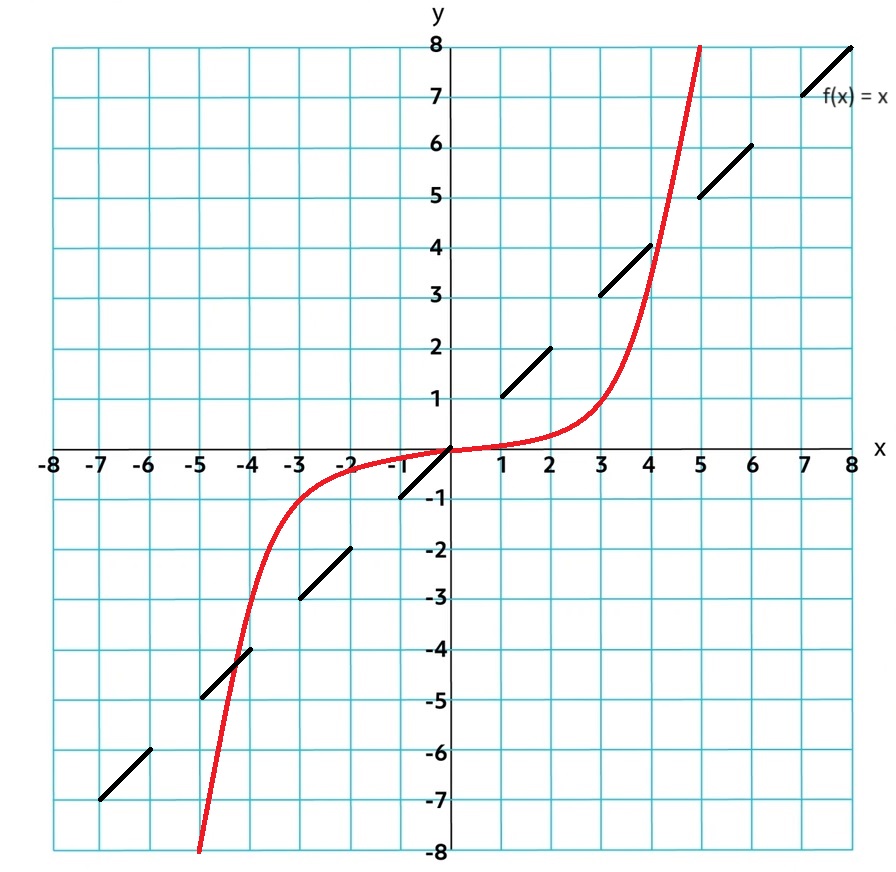
If the function is odd it have symmetry across the origin. f(-x) = -f(x)

1.6 Polynomial Functions and End Behavior

1.6.A

Behavior of Polynomial Functions: As input values increase or decrease without bound, the ouput values will either increase of decrease without bound. In the notation: (said: Limit of f(x) as x approaches ∞/-∞ is equal to ∞/-∞)

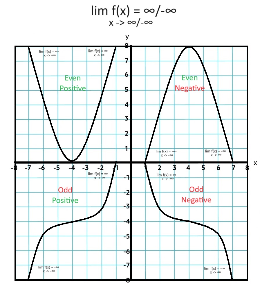
The degree and sign of the leading term effect the end behavior of the polynomial function.

1.7 Rational Functions and End Behavior

1.7.A

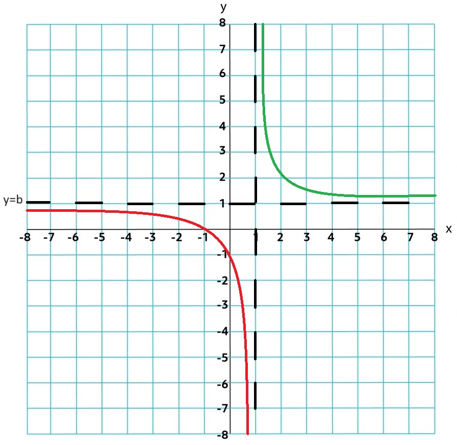
Rational Function: f(x) = p(x)/q(x) = a polynomial/ a polynomial. The end behavior of the function will be affected by the polynomial with a greater degree.

^p(x)⁄_q(x)

p(x) < q(x) : HA at y=0

p(x) > q(x) : No HA

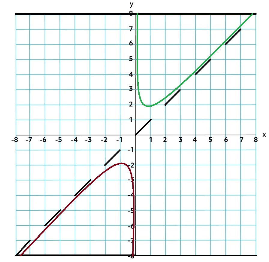
p(x) - 1 = q(x) : oblique/slant

p(x) = q(x) : HA = Numerator coefficient/ Denominator coefficient

Limit Notation: Lim r(x) = b; x → ∞ or Lim r(x) = b; x → -∞

1.8 Rational Functions and Zeros

1.8.A

Real Zeros: Found in the Numerator for values in its domain

The real zeros of both polynomial functions of a rational function r are endpoints or asymptotes for intervals satisfying the rational function inequalities: r(x) > 0 or r(x) < 0

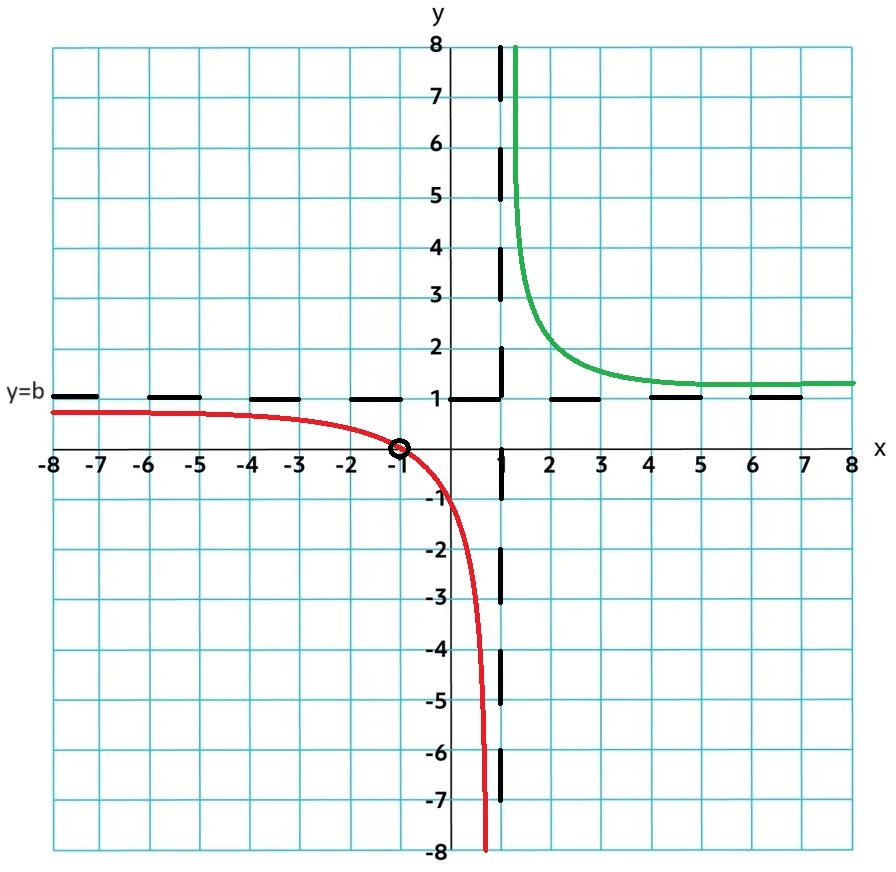
r(x) > 0: (-∞,-1] ∪ [1, ∞)

r(x) < 0: (-1, 1)

1.9 Rational Functions and Vertical Asymptotes

1.9.A

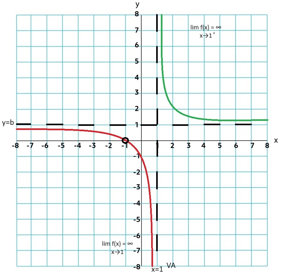
Vertical Assymptote: Real Zeros Found in the Denominator of a Rational Function. It is a VA if its multiplicity is greater than the real zero in the numerator.

Limit Notation: x=a of a rational function, the values of the polynomial function in the denominator are arbitrarily(extremly close) close to zero, so the values of the rational function r increase or decrease without bound.

lim r(x) = ∞; x→a⁺ or lim r(x) = −∞; x→a⁺ for near a and greater than a for input values near a and greater than a (from the right side)

lim r(x) = ∞; x→a^- lim r(x) = −∞; x→a^- for input values near a and less than a (from the left side)

1.10 Rational Functions and Holes

1.10.A

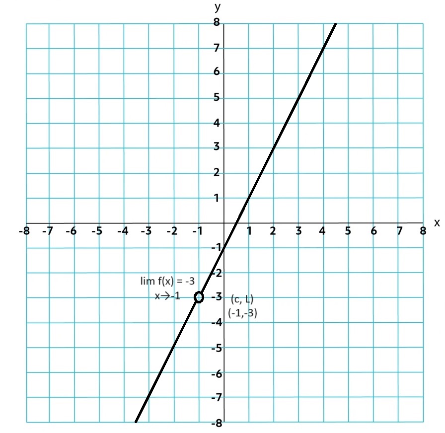
If the multiplicity of a real zero in the numerator is greater than or equal to its multiplicity in the denominator, then the graph of the rational function has a hole at the corresponding input value.

f(x) = ^2x2+x-1⁄_x+1

If the hole is at x = c, the hole has a coordinate (c, L)

lim r(x) = ∞; x→a

1.11 Equivalent Representations of Polynomial and Rational Expressions

1.11.A

Factored Form: Provides information about real zeros, it can reveal information about x-intercepts, asymptotes, holes, domain, and range

f(x) = ^(x-3)(x+5)⁄_(x-6)(x+2)

Standard Form: can reveal information about end behavior.

f(x) = ^x2+2x-15⁄_x²-4x-12

1.11.B

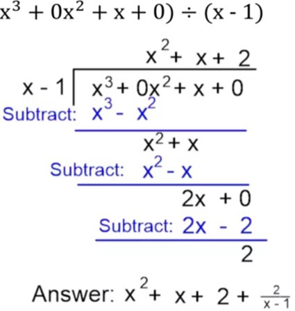
Polynomial Long Division: f is divided by g, rewritten as f(x) = g(x)q(x) + r(x), where q is the quotient, r is the remainder, and the degree of r is less than the degree of g. The quotient can be used to find slant assymptotes for rational functions

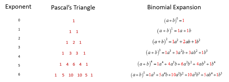
Pascals Triangle: easily expand expressions of the form (a+b)ⁿ, including polynomial functions of the form p(x) = (x+c)ⁿ, where c is a constant

1.12 Transformations of 3 Functions

1.12.A

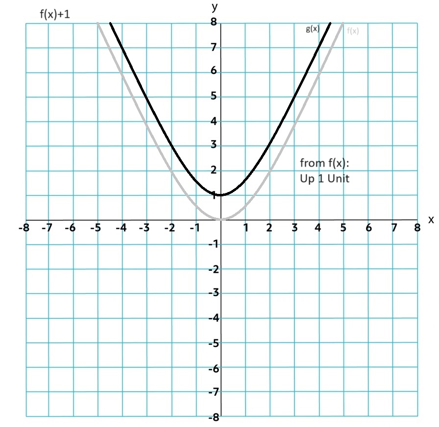
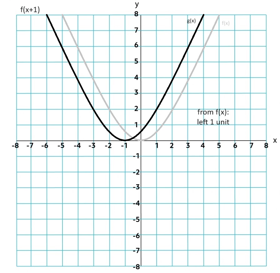
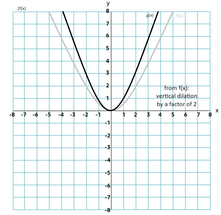
Transformations: g(x)=a f(b(x+h))+k

k is a vertical translation of f by k units

h is a horizontal translation of f by -h units

a is a vertical dilation by a factor of |a|. If a is negative it is a reflection over the x-axis

b is a vertical dilation by a factor of |¹⁄_b|. If b is negative it is a reflection over the y-axis

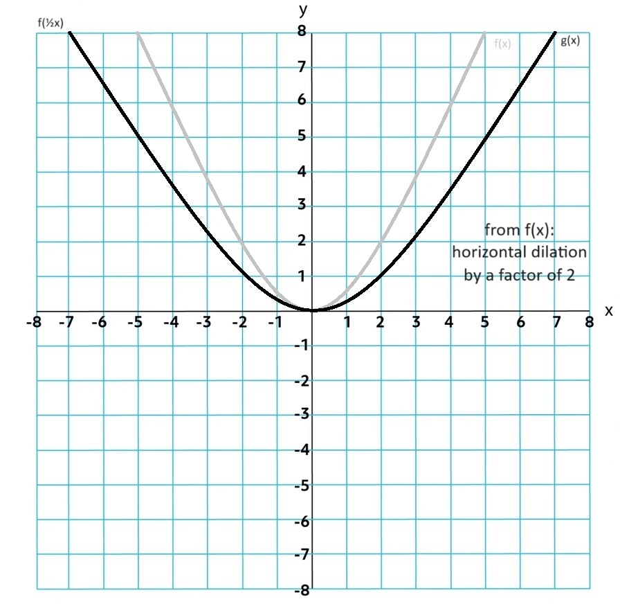
!!!The Domain and Range can change from the parent function!!!

1.13 Function Model Selection and Assumption Articulation

1.13.A

Linear functions: model data sets or aspects of contextual scenarios that demonstrate roughly constant rates of change.

Quadratic functions: model data sets or aspects of contextual scenarios that demonstrate roughly linear rates of change, or data sets that are roughly symmetric with a unique maximum or minimum value.

Geometric: contexts involving area or two dimensions can often be modeled by quadratic functions. Geometric contexts involving volume or three dimensions can often be modeled by cubic functions.

Polynomial functions model data sets or contextual scenarios with multiple real zeros or multiple maxima or minima. The degree n models data sets or contextual scenarios that demonstrate roughly constant nonzero nth differences in polynomial functions. With a degree n or less you can model a graph of n + 1 points with distinct input values

A piecewise function consists of a set of functions defined over nonoverlapping domain intervals and is useful for modeling a data set or contextual scenario that demonstrates different characteristics over different intervals

1.13.B

A model may have underlying assumptions about what is consistent in the model.

A model may have underlying assumptions about how quantities change together.

A model may require domain restrictions based on mathematical clues, contextual clues, or extreme values in the data set.

A model may require range restrictions, such as rounding values, based on mathematical clues, contextual clues, or extreme values in the data set.

1.14 Function Model Construction and Application

1.14.A

A model can be constructed based on restrictions identified in a mathematical or contextual scenario. It can also be contructed by using transformations of the parent function. Can be modeled by using a calculators linear, quadratic, cubic and quartic regressions.

Piecewise function: can be contructed through various modeling techniques

1.14.B

Rational Function: can graph quantities that are inversely proportional.

y=^k⁄_x

k = constant of porportionality

1.14.C

A model can be drawn by answering key questions and predicting values, rates of change, average rates of change, and changing rates of change. Use appropiate units of measurment given from the context.